Machine Learning
这是第一份机器学习笔记,创建于2019年7月26日,完成于2019年8月2日。
该笔记包括如下部分:
- 引言(Introduction)
- 单变量线性回归(Linear Regression with One Variable)
- 线性代数(Linear Algebra)
- 多变量线性回归(Linear Regression with Multiple Variables)
- Octave
- 逻辑回归(Logistic Regression)
- 正则化(Regularization)
Part 1 :Introduction
- Machine Learning:
- Idea:
- 给予机器自己学习解决问题的能力
- 先得自己搞明白了才有可能教会机器自己学习呐。。
- Machine learning algorithms:
- Supervised learning
- Unsupervised learning
- Others: Recommender systems(推荐系统) ; Reinforcement learning(强化学习)
- Supervised learning(监督学习)
-
Use to do :
- Make predictions
-
Feature:
- Right answers set is GIVEN
-
Including:
- Regression problems(回归问题)
我们给出正确的数据集,期望算法能够预测出continuous values(连续值)。 - Classification problems(分类问题)
我们给出正确的数据集,期望算法能够预测出discrete valued(离散值) 。
(the features can be more than 2 , Even infinite.)
- Regression problems(回归问题)
- Unsupervised learning(无监督学习)
-
Feature:
- We just give the data and hope it can automatically find structure in the data for us.
-
Including:
- Clustering algorithms(聚类算法)
-
Problems:
- In fact I find the unsupervised learning looks like the classification problems . The only difference is whether or not the data set is GIVENGive the correct data ahead of time .
-
Summary:
- We just give the Disorderly data sets , and hope the algorithm can automatically find out the structure of the data , and divide it into different clusters wisely.
- Octave
Usage:
- 用octave建立算法的原型,如果算法成立,再迁移到其他的编程环境中来,如此才能使效率更高。
Part 2 :单变量线性回归(Linear Regression with One Variable)
- 算法实现过程:
- Method:
- Training set Learning algorithm hypothesis function(假设函数) Find the appropriate form to represent the hypothesis function
-")
- Training set Learning algorithm hypothesis function(假设函数) Find the appropriate form to represent the hypothesis function
- 简单来说就是我们给出Training Set , 用它来训练我们的Learning Algorithm ,最终期望能够得到一个函数 h(theta), 这也就是预测的模型,通过这个模型,我们能够实现输入变量集,然后就能够返回对应的预测值。
- Cost function(代价函数)
-
关于h(x)函数
- 对于房价问题,我们决定使用Linear function 来拟合曲线 ,设 h(x)= theta(0)+theta(1)* x
- 因为我们最后想要得到的就是 h(x),对于 x 来说,它是始终变化的,每一条数据对应着不同的变量集,无法固定;所以algorithm想要确定的就是不变的量 theta集 了。在以后的操作中,因为我们想要求得的是 theta集,所以更多的时候,我们会把 x 看作是常量,却把 theta 看作是变量,所以一定不要糊涂了。
-
建模误差(modeling error)
- 我们选择的参数决定了我们得到的直线相对于我们的训练集的准确程度,模型所预测的值与训练集中实际值之间的差距就是建模误差(modeling error)。
Description:
- Cost function sometimes is also called squared error function(平方误差函数)
- Cost function 用于描述建模误差的大小。
一般来说,误差越小,Cost function 就能够更好的与数据集相拟合,但这并不是绝对的,因为这有可能会产生过拟合问题。 -
")
把它进一步的拆开来看就应该是这样子的:J( theta(0),theta(1) ) = 1/2m * Sigma [1-m] {theta(0)+theta(1)* x(i) - y(i)}(可能就我一人能看懂。。) - 平方误差函数只是 Cost function 中的一种形式。在这里我们之所以选择squared error function , 是因为对于大多数问题,特别是回归问题,它是一个合理的选择。还有其他的代价函数也能很好地发挥作用,但是平方误差代价函数可能是解决回归问题最常用的手段了。
- Gradient descent(梯度下降) algorithm
-
Idea:
- 我们已经知道了,**h(theta)**是用来拟合数据集的函数,如果拟合的好,那么预测的结果不会差。J(theta集)被称为代价函数,如果代价函数较小,则说明拟合的好。而此时的theta集就是我们就是问题的解了。
- 我们已经知道了我们的目标theta集,那么如何求得theta集呢?
- Gradient descent!
-
Usage:
- Start with some para0,para1…
- Keep changing paras to reduce J (para0,para1) to find some local minimum
- Start with different parameters , we may get different result
- (所以,我们保证J(theta集)与各个theta构成的函数是一个凸函数,换句话说保证存在唯一的极小值=极小值)
- Until we hopefully end up at a minimum
-
Formula:
批量梯度下降公式
")
<a> is learning rate which control how big a step we use to upgrade the paras.
So if the <a> is too small , the algorithm will run slowly ; but if <a> is too big , it can even make it away from the minimum point .
另外,每次theta下降的幅度都是不一样的,这是因为实际上theta每次下降多少是由 【<a>*Derivative Term】这个整体决定的,<a>是下降幅度的重要决定因子,但并不是全部。
在每次下降以后,Derivative Term都会变小,下一次下降的幅度也会变小,如此,控制梯度慢慢的下降,直到Derivative Term=0。the rest of the formula is the Derivative Term(导数项) of theta
In this image,we can find that no matter the Derivative Term of theta is positive or negative , the Gradient descent algorithm works well
")
the Details of the formula:
")
Attention:
With the changing of the paras,the derivative term is changing too.
So:
Make sure updating the paras at the same time.(simultaneous update同步更新)
For what? Because the derivative should use the former para rather than the new.
How:
在全部theta没有更新完成之前,我们用temp集来暂时存储已经更新完成的theta集,直到最后一个theta也更新完成之后,我们才再用存储在temp集里的新theta集更新原theta集。
- Gradient descent for linear regression
-
“Batch” Gradient descent :
- Each step of gradient descent uses all the training examples .
- 在梯度下降公式中存在某一项需要对所有m个训练样本求和。
-
Idea:
- 将梯度下降与代价函数相结合
")
-
The result:
")
- This is the result after derivation. And we can find that comparing with the first formula , the second has a x term at the end . It does tell us something that the variable is para0 and para1 , not the x or y . Although they looks more like variables.
- After derivation , for the first formula we have nothing left , for the second , we just has a constant term(常数项) x left .
-
Finally:
- We have other ways to computing J(theta):
- 正规方程(normal equations),它可以在不需要多步梯度下降的情况下,也能解出代价函数的最小值。
- 实际上在数据量较大的情况下,梯度下降法比正规方程要更适用一些。
Part 3 :线性代数(Linear Algebra)
矩阵和向量提供了一种有效的方式来组织大量的数据,特别是当我们处理巨大的训练集时,它的优势就更加的明显。
- Matrices and vectors (矩阵和向量)
-
Matrix:
- Rectangular array of numbers.
- 二维数组
-
The dimension(维度) of the matrix :
- number of row * number of columns
-
Matrix Elements :
- How to refer to the element
")
- How to refer to the element
-
Vector:
- An n*1 matrix . ( n dimensional vector. n维向量)
- How to refer to the element in it
- We use 1-indexed vector
-
Cvention:
- We use upper case to refer to the matrix and lower case refer to the vector.
- Addition and scalar multiplication (加法和标量乘法)
- 行列数相等才能进行加法运算:
- 标量与矩阵的乘法:
")
")
- Matrix-vector multiplication(矩阵-向量乘法)
Details:
")
- A’s row number must be equal with B’s column number .
- Matrix-matrix multiplication(矩阵-矩阵乘法)
- Details:
")
- Just as matrix-vector , the most important thing is to make sure A’s columns number is equal with B’s rows number .
- C’s columns number is equal with B’s .
- n fact , before multiply between Matrixs , we can divide B into several vectors by columns, and then we can make the Matrix- Vector multiplication.
- A column of B corresponding a hypothesis , and a column of C corresponding a set of prediction .
- Matrix multiplication properties(矩阵乘法特征)
-
Properties :
- Do not enjoy commutative property(不遵循交换律)
- Enjoy the associative property(遵循结合律)
-
Identity Matrix(单位矩阵):
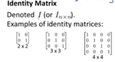Feature:
它是个方阵,从左上角到右下角的对角线(称为主对角线)上的元素均为1。除此以外全都为0。它的作用就像是乘法中的1。Usage:
is the identity matrix .
A(m , n) * I(n , n) = I(m , m) * A(m , n)
M1’s column number should be equal with M2’s row number .
- Matrix inverse operation(矩阵的逆运算)
- Attention:
")
- Only square matrix have inverse .
- Not all number have inverse , such as 0 .
- Matrix transpose operation(矩阵的转置运算)
- Definition:
- Official definition:
")
即将A与B的x , y坐标互换 - 矩阵转置的基本性质:
")
")
Part 4:多变量线性回归(Linear Regression with Multiple Variables)
在之前的部分中,学习了单变量/特征的回归模型。在这一部分进行深入,将变量的数量增加,讨论多变量的线性回归问题。
- Multiple feature(多功能)
- Example:
")
对于新问题的注释:
")
- So the final prediction result is a vector too .
- 可以发现,多变量线性回归和单变量线性回归基本是一样的,唯一的变化就是theta变成了theta集;变量x变成了x集。
- Gradient descent for multiple variables(多元梯度下降法)
-
Idea:
- 与单变量线性回归类似,在多变量线性回归中,我们也构建一个代价函数,则这个代价函数是所有建模误差的平方和
- 代价函数:
")
- 梯度下降法应用到代价函数并求导之后得到:
")
-
Feature scaling(特征缩放):
- Purpose:
Make the gradient descent runs faster .
尤其是如果我们采用多项式回归模型,在运行梯度下降算法前,特征缩放非常有必要。 - Idea:
Make sure number are in similar scale . - Usage:
")
- The range limit :
Get every feature range from -3 to 3 or -1/3 to 1/3 . That’s fine .
In fact there is no problems , because the feature is a real number ! That’s means it will never change .
x 是变量,并且它是已知的,我们可以从data set 中直接获得,我们可以对它进行特征缩放;theta是未知的,是我们要求的目标。
- Purpose:
-
Summary:
- 特征缩放缩放的是 已知的 变量x ,而不是 未知的 常量theta 。
- 进行特征缩放是为了为了提高梯度下降的速度。
- Learning rate (学习率)
- Idea:
- If the gradient descent is working properly , then J should decrease after every iteration.
- 梯度下降算法收敛所需要的迭代次数根据模型的不同而不同,我们不能提前预知,我们可以绘制迭代次数和代价函数的图表来观测算法在何时趋于收敛。
- Convention:
- 通常可以考虑的学习率<a>的数值:
0.01;0.03;0.1;0.3;1;3;10;
- 通常可以考虑的学习率<a>的数值:
- Summary:
- If <a> is too small slow move
- If <a> is too big J may not decrease on every iteration .
- Features and Polynomial regression(多变量和多项式回归)
Idea:
- Linear regression 并不适应所有的数据模型,有时我们需要曲线来适应我们的数据,比如一个二次方模型:
- 通常我们需要先观察数据再确定最终的模型
Attention:
- 如果我们采用多项式回归模型,在运行梯度下降算法前,特征缩放非常有必要。
- Normal equation(常规方程)
-
Idea:
- 从数学上来看,想要求得J(theta) 的最小值,最简单的方法就是对它进行求导,令它的导数=0,得出此时的theta就是最终的结果
- 而正规方程方法的确就是这么干的
-
Attention:
- 对于那些不可逆的矩阵(通常是因为特征之间不独立,如同时包含英尺为单位的尺寸和米为单位的尺寸两个特征,也有可能是特征数量大于训练集的数量),正规方程方法是不能用的。
- 这就是正规方程的局限性
Usage:
")
- Example:
")
")
")
")
- The Comparison of Gradient descent and Normal equation
Gradient descent :
- Need to choose
- Need many iterations
Normal equation :
- Need to compute [x’*x]^(-1) , So if n is large it will run slowly .
- Do not fit every situations (只适用于线性模型,不适合逻辑回归模型等其他模型).
Summary:
- 只要特征变量的数目并不大,标准方程是一个很好的计算参数的替代方法。具体地说,只要特征变量数量小于一万,我通常使用标准方程法,而不使用梯度下降法。
- Normal equation 不可逆情况
Idea:
")
- 第一要降低features之间的相关度
- 第二要适当的减少features 的数量
")
Idea:
")
Part 5:Octave教程(Octave Tutorial)
Part 6:逻辑回归(Logistic Regression)
- Vectorization(矢量化)
- Example:
")
使用向量的转置来求两个向量的内积,可以非常方便的处理大量的数据。
这就是所谓的矢量化的线性回归。
- Classification(分类问题)
- Convention in Classification problems:
0 equal to empty ;
1 means something is there. - Attention:
In classification problems , we want to predict <离散值>
- Hypothesis Representation(假说表示)
-
Question:
- What kind of function we need to use to represent our hypothesis in the classification problems?
- Linear function image may out of the range[-1,1]
-
Idea:
- Make sure
")
- Make sure
-
Import :
- Logistic regression(逻辑回归)
-
Hjypothesis:
")
-
Status:
- The most popular machine learning algorithm.
- 一种非常强大,甚至可能世界上使用最广泛的一种分类算法。
Attention:
Although we called it ‘regression’ , but in fact it is used in classification
Problems.Logistic function:
")
")
")
- Decision boundary
- 决策边界不是训练集的属性,而是假设本身以及其参数的属性;所以说
只要给定了theta那么决策边界就已经确定了。(theta集确定了,那么函数就确定了,决策边界自然也就被确定了)- 训练集–>生成theta–>确定决策边界
- Logistic Regression Cost function(逻辑回归的代价函数)
-
Question:
- How to choose parameter theta?
- 因为我们改变了代价函数的模型h(theta) ,这样J(theta)-theta 的函数图像就会由许多个极小值,这对于我们求得theta是不利的
-
Idea:
为了保证Cost function 是凸函数,我们选择更换代价函数。
在当时学代价函数的时候就直到,代价函数并不只是有一种形式。实际上代价函数只是为了表征误差的的大小,所以只要是能够合理的表示误差的函数都可以当作是误差函数。
")
Simplified cost function:
")
基于只有y=1 || y=0 两种情况横坐标表示的是h(x) ,也就是我们的模型得出来的 y 值 , 纵坐标是Cost function,对于 y=1 和 y=0 有不同的图像的,这两个图像都是在一端等于0 , 在另一端趋于无穷大。
")
- Logistic Regression Gradient Descent(逻辑回归的梯度下降)
-
Idea:
- 我们已经找到了合适的Cost function 了 ,现在就可以使用它进行梯度下降了
-
Details:
- 对于梯度下降,无论Cost function 是什么 ,它的 algorithm是始终不变的
")
- 我们将Cost function 带入, 结果如下:
")
- 对于梯度下降,无论Cost function 是什么 ,它的 algorithm是始终不变的
-
Attention:
- 虽然得到的梯度下降算法表面上看上去与线性回归的梯度下降算法一样,但是这里的 h(x)与线性回归中不同(此处的是逻辑回归函数而之前的是线性函数)所以实际上逻辑函数的梯度下降,跟线性回归的梯度下降是两个完全不同的东西。
- 另外,在运行梯度下降算法之前,进行特征缩放依旧是非常必要的。
一些梯度下降算法之外的选择: 除了梯度下降算法以外,还有一些常被用来令代价函数最小的算法,这些算法更加复杂和优越,而且通常不需要人工选择学习率,通常比梯度下降算法要更加快速。这些算法有:共轭梯度(Conjugate Gradient),局部优化法(Broyden fletcher goldfarb shann,BFGS)和有限内存局部优化法(LBFGS) ,fminunc是 matlab和octave 中都带的一个最小值优化函数,使用时我们需要提供代价函数和每个参数的求导,下面是 octave 中使用 fminunc 函数的代码示例:
function [jVal, gradient] = costFunction(theta)
jVal = [...code to compute J(theta)...];
gradient = [...code to compute derivative of J(theta)...];
end
options = optimset('GradObj', 'on', 'MaxIter', '100');
initialTheta = zeros(2,1);
[optTheta, functionVal, exitFlag] = fminunc(@costFunction, initialTheta, options);
%很醉人,这谁佛得了啊
- Advanced Optimization(高级优化)
雾里看花。。。
- 梯度下降并不是我们求theta最好的方法,还有其他一些算法,更高级、更复杂。
- 共轭梯度法 BFGS (变尺度法) 和L-BFGS (限制变尺度法) 就是其中一些更高级的优化算法
- 优点:
通常不需要手动选择学习率 ;
算法的运行速度通常远远超过梯度下降。
- 优点:
- Octave代码实现:
%定义Cost function 函数

function [jVal, gradient]=costFunction(theta)

  jVal=(theta(1)-5)^2+(theta(2)-5)^2;

  gradient=zeros(2,1);

  gradient(1)=2*(theta(1)-5);

  gradient(2)=2*(theta(2)-5);

end
- 调用该函数:
")
你要设置几个options,这个options变量作为一个数据结构可以存储你想要的options,

所以 GradObj 和On,这里设置梯度目标参数为打开(on),这意味着你现在确实要给这

个算法提供一个梯度,然后设置最大迭代次数,比方说100,我们给出一个 的猜测初始

值,它是一个2×1的向量,那么这个命令就调用fminunc,这个@符号表示指向我们刚刚

定义的costFunction 函数的指针。如果你调用它,它就会使用众多高级优化算法中的一

个,当然你也可以把它当成梯度下降,只不过它能自动选择学习速率,你不需要自己来

做。然后它会尝试使用这些高级的优化算法,就像加强版的梯度下降法,为你找到最佳

的值。
学到的主要内容是:写一个函数,它能返回代价函数值、梯度值,因此要把这个应用到逻辑回归,或者甚至线性回归中,你也可以把这些优化算法用于线性回归,你需要做的就是输入合适的代码来计算这里的这些东西。
- Multiclass Classification_ One-vs-all (多类别分类:一对多)
Part 7:正则化(Regularization)
有时我们将我们的算法应用到某些特定的机器学习应用时,通过学习得到的假设可能能够非常好地适应训练集(代价函数可能几乎为0),但是可能会不能推广到新的数据。这就是过拟合(over-fitting)的问题。
正则化(regularization)的技术,它可以改善或者减少过度拟合问题。
- 处理过拟合问题的思路
- 丢弃一些不能帮助我们正确预测的特征。可以是手工选择保留哪些特征,或者使用一些模型选择的算法来帮忙(例如PCA)
- 正则化。 保留所有的特征,但是减少参数的大小(magnitude)。
- 处理过拟合问题的代价函数
- Idea:
- 过拟合问题的产生很大程度上是由于高次项。所以为了避免过拟合问题,我们要做的就是对高此项进行限制,具体做法就是在代价函数里对他们施加惩罚。
- 在一定程度上减小这些参数theta的值,这就是正则化的基本方法。
- 例如:
")
- 假如我们有非常多的特征,我们并不知道其中哪些特征我们要惩罚,我们将对所有的特征进行惩罚,并且让代价函数最优化的软件来选择这些惩罚的程度。这样的结果是得到了一个较为简单的能防止过拟合问题的假设,就像这样:
")
其中lambda又称为正则化参数(Rguarization Parameter)。 注:根据惯例,我们不 theta0进行惩罚。- **lamnda **
38.Regularized Linear Regression(正则化线性回归)
- 正则化线性回归的代价函数为:
")
- 如果我们要使用梯度下降法令这个代价函数最小化,因为我们不对theta0进行正则化,所以梯度下降算法将分类讨论,对theta0特殊处理。
- 我们对方程进行拆解,可以看出,实际上正则化线性回归的梯度下降算法的变化在于,每次都在原有算法更新规则的基础上令值减少了一个额外的很小的值。
")
- 正规方程来求解正则化线性回归模型:
")
- Regularized Logistic Regression (正则化逻辑回归模型)
- 仿照线性回归正则化的思路,我们只需要修改代价函数,添加一个正则化的表达式即可:
")